Introduction:

Stars having a mass more than 11 Solar Masses undergo core-collapse supernova explosion, and leaves behind a compact object, either a neutron star or a black hole, which would depend on the initial mass and the initial metallicity of the progenitor star. In this project, I have explored the mass distribution function of the Fe core and inner shell masses using the MESA stellar code. The work is based on the work by Timmes.et.al[1].

Parameter Exploration

• Initial Mass: [16-50] Solar Masses.
• Initial Metallictiy: [10^-4 , 10^-3, 10^-2 , 10^-1]

Mesa Models:

I used the following MESA models for the study:

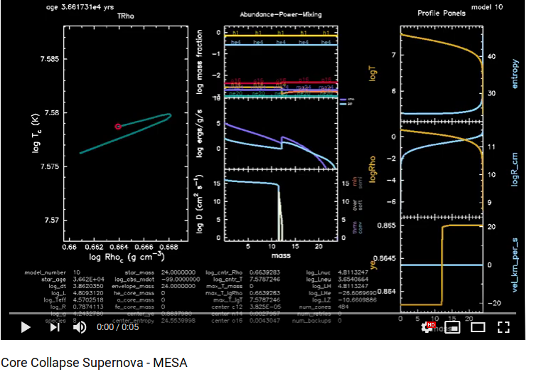
1. 25M_pre_ms_to_core_collapse*: This model evolves a pre-main sequence star and terminates when the Fe core starts to fall in with a rate higher than a threshold value. One can look at this models evolution in the video below for a 24 solar mass star with z=0.01.

• One can see how the star burns the hydrogen in its core to He, and then He to carbon and oxygen, and then to heavier elements in a shell-like structure. The abundance plot shows this shell-like distribution and burning of isotopes.
• From the Ye plot, we can see the separation between hydrogen layer and He layer.
• At the end of the simulation, the Ye near the center of the star falls, showing the formation of neutron-rich isotopes, which in this case is mostly Fe56.
• This model uses a 21 isotope nuclear reaction network.

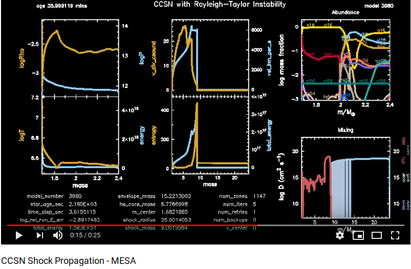
2. example_ccsn_IIp: This model takes the saved model from the “25M_pre_ms_to_core_collapse” run and advances a shock, which burns the inner shell elements. This model was used to compute the fallback mass onto the remnant, which would increase its final mass, which could go beyond the Si shell.

• The variable parameter for this model is the amount of energy deposited at the edge of the Fe core. This value was set to 1.56e51 ergs.
• Out of 97 models only 25 “25M_pre_ms_to_core_collapse” converged to a final state.
• One can see the propagation of shock and the nucleosynthetic yields(from Progenitor mass=24, Z=0.01 model) in the video below:

Computational Framework:

To explore such a big parameter space, running individual models is not feasible, so I developed a framework where I could submit multiple models over a set of compute nodes on Carnie, to parallelly compute multiple models at the same time (UMass Dartmouth computer cluster).

• The parameter space has [number(Initial_masses) X number(Initial_metallicity)] points, is subdivided into sets of 15 models per set.
• For each set, a separate directory is created, which will contain separate directories for each of its models.
• Each of these set directories contains a copy of the directory “25M_pre_ms_to_core_collapse”. The directory name is marked with a label M__Z.
• Each of these model directories has an initial_mass and initial_z in the “inlist_common” file. These values are varied for each model, by making use of templates.
• Each model directory is compiled using by executing ‘./mk’.
• Each set directory also contains an SBATCH submission script(to be run on a single node), which will execute the ‘./rn’ inside each of the model directories in order.
• I created a total of 20 sets. Each set was submitted to a particular node having 48 hardware threads(24 cores).
• Codes: create_param_sets.py, execute_run.py, create_IIp_param.py,execute_IIp_run.py, execute_jobs.py

Chandrasekhar mass for Neutron Stars:

• M_ch ~ M_ch0[1 + (Se/pi*Ye)^2]
  • Se: Electronic entropy per baryon.
  • Ye: Charge fraction Z/A
• Se: This is proportioanl to the Mass of the Iron core, which is in proportional to the mass of the progenitor star.

From these relations, we expect that higher mass main sequence stars will have a massive Fe core. Also, a higher metallicity value will have a lower Ye value, which would give a higher value of the M_ch. (From [1])

Results:

Looking at the results from the simulation runs:

Fe Core vs. Initial Mass

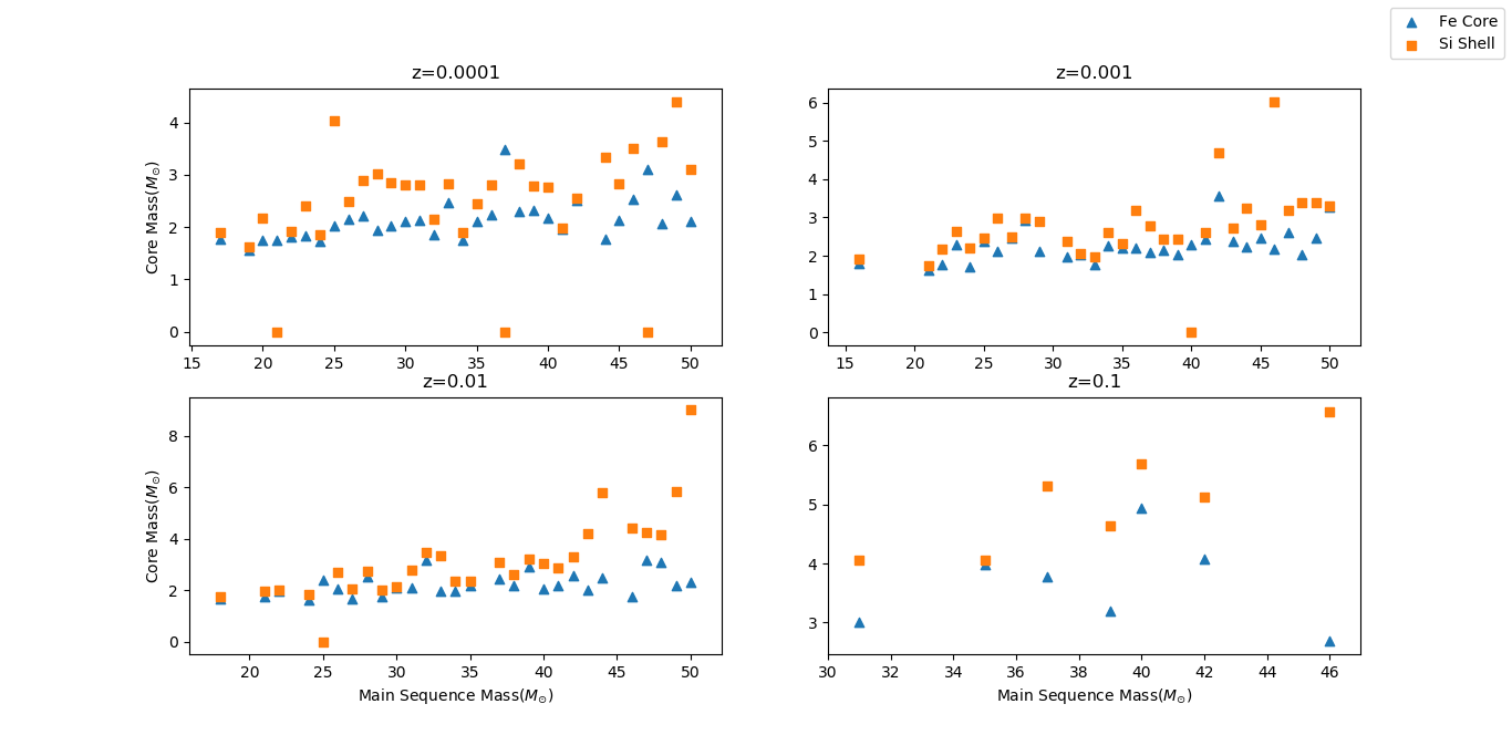
• The following is a scatter plot showing the Fe core masses in the blue triangle and the Si shell masses in the orange square for each of the 97 models. -Each separate plot shows a different metallicity value shown at the top of the subplot.
• We can see from the plots, that for a fixed metallicity value, the Fe core and Si shell mass increases with progenitor mass, which is what we would expect.
• Further, we can see that for higher values of metallicity we have a higher Fe core and Si shell mass. Because of the inverse relation with Ye.

Core mass and its effect on Metallicity

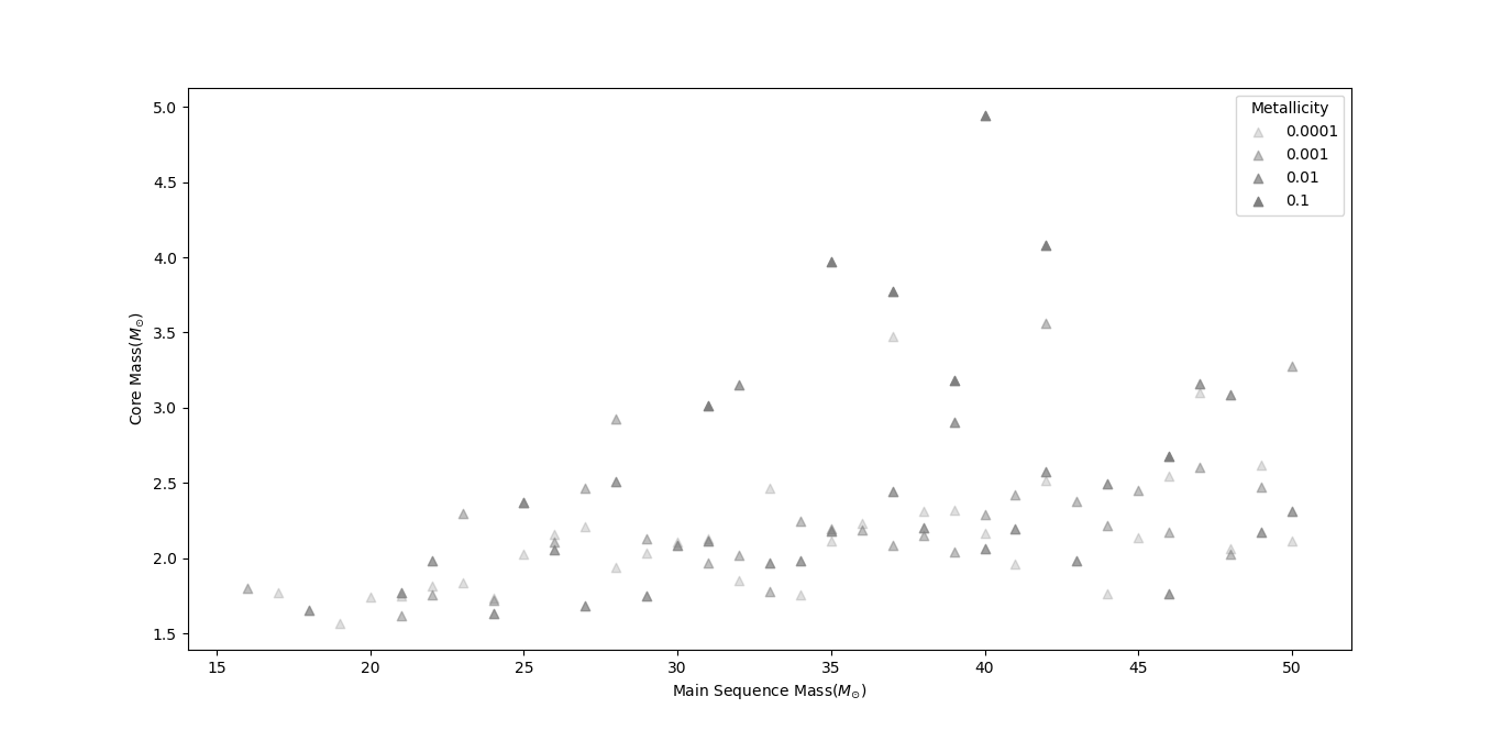
• This plot shows the Fe core mass vs. progenitor mass of each model. The grayscale shade of the data point represents the metallicity of that model.
• We can see that a higher metallicity for the same progenitor mass will have a more massive Fe core, something that we would expect from the mass and Ye relation.
• Further, we can say that the points above the max mass limit of a neutron star(~3 solar masses) will all be black holes. Of course, points below 3 solar masses can be black holes, which depends on how much matter fell back onto the remnant.

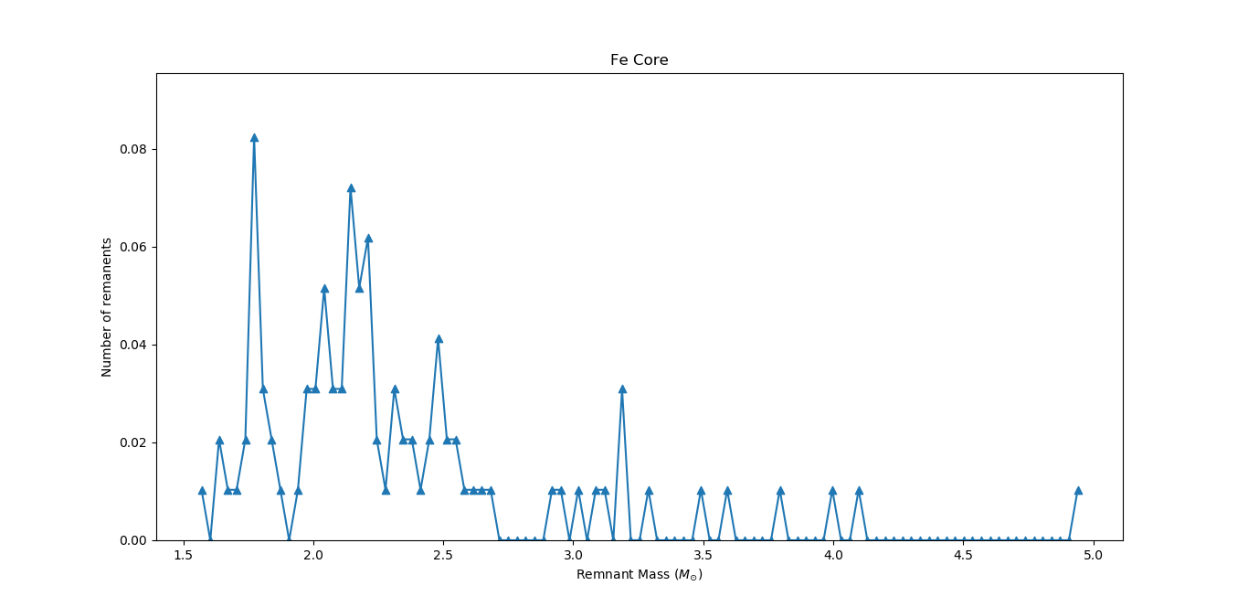
Fe Core Distribution Function

• From the Fe core masses of the models, we can make a distribution function of the number of remnants in a particular mass range.
• The following plots show this distribution of Fe core masses. Here the bin size of the remnants 0.035 solar masses.
• We can observe peaks at ~1.8 solar masses and another around 2.3 solar masses. Timmes.et.al[1] get a similar valued peak at around 1.6 solar masses. They also get a major peak at 1.2 solar masses, which is not in this plot. This is because the “pre_ms_to_core_collapse” model failed to converge for masses [11-16] solar masses, which would have given this 1.2 solar mass peak. -Code: analysis.py

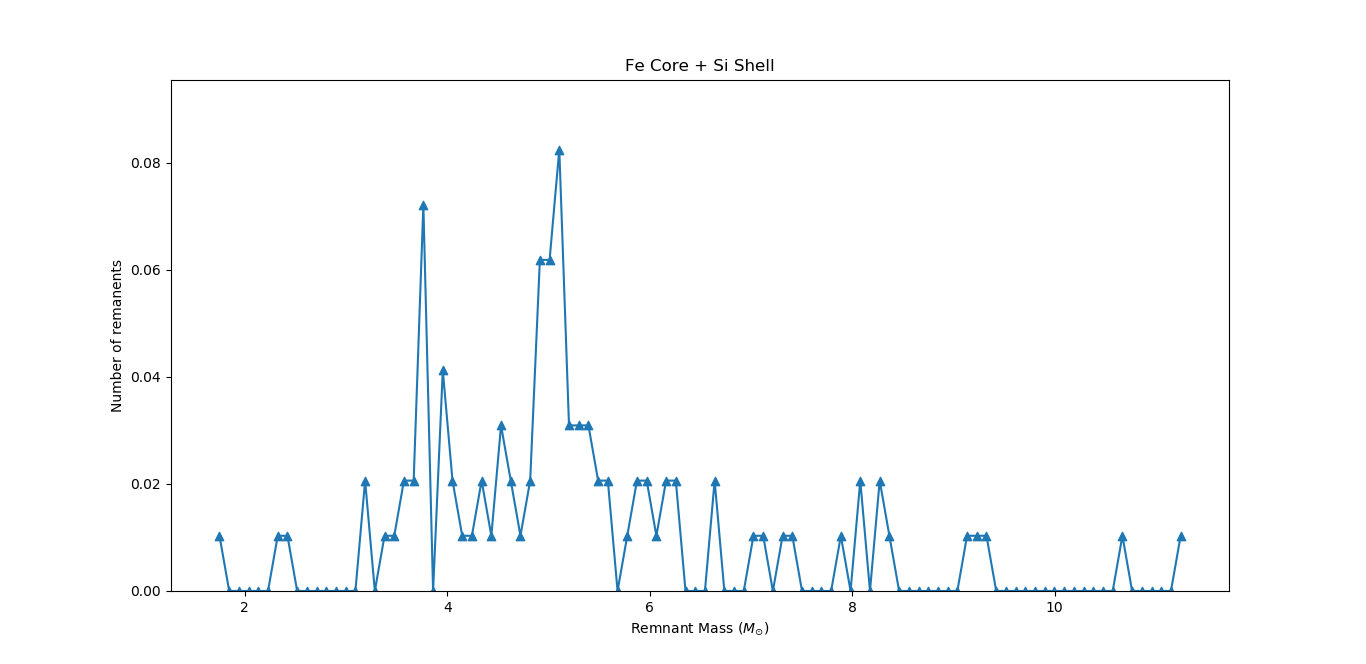
Fe Core + Si Shell Distribution Function

• Similar mass distribution, with the addition of Si shell mass to the model.

Final Remnant Mass

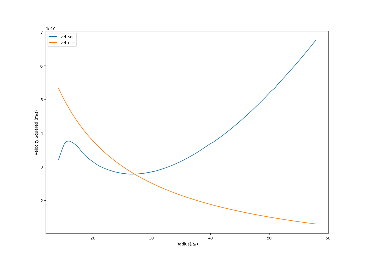
• To calculate the final remnant mass, I estimated how much mass would be bound to the star. To do this, I calculated the escape velocity as a function of radius and compared that with the velocity of the ejecta at that radius.
• V_esc = sqrt(2GM_in/r_in)
• If the velocity at that radius is less than the escape velocity, the mass interior to that location is bound and will fall onto the remnant.
• The following graph shows the square of the escape velocity and the square of ejecta velocity, for a model (M=29 Solar mass, Z=0.01). Mass interior to the intersection of the curves gives the fallback mass.
• Code: last_plot.py

Final remnant Mass vs. Main Sequence Mass

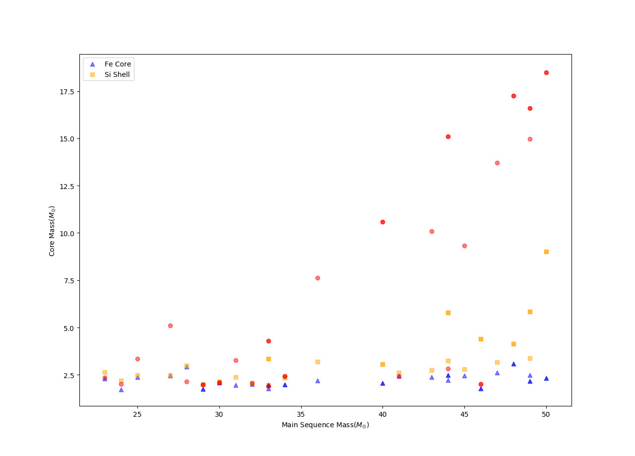
• Mass calculated using the above method is plotted on the scatter plot shown below.
• One can see that for some of the low progenitor mass, the fallback is less than the Si shell mass.
• For high mass progenitors, a large amount falls back into the remnant, as seen from the plot.
• This is probably because of the energy deposition on the Fe core edge(~ 1.5 10^51 erg).
• As low mass stars are more loosely bound as compared to the higher mass stars. For the same energy, the shock can unbind large mass fractions as compared to the more massive stars.

Conclusion

In the project, I evaluated the mass distribution function of CCSN remnants by calculating 97 mesa models over the parameter space of initial progenitor mass and metallicity. The distribution showed a major peak in the Fe core distribution function at ~1.8m solar masses, which is very close to the second peak in timmes.et.al[1] paper. Further, I saw an addition peak of ~2.3 solar mass. Further, I explored the effects of initial progenitor mass and its initial metallicity on remnant masses. I saw a correlation between remnant mass and progenitor mass. A similar correlation was found for initial metallicity and is something that was expected from the Chandrashekar mass formula.

References:

[1] Timmes, F. X., S. E. Woosley, and Thomas A. Weaver. “The neutron star and black hole initial mass function.” arXiv preprint astro-ph/9510136 (1995).

[2] Woosley, S. E., and Thomas A. Weaver. The evolution and explosion of massive Stars II: Explosive hydrodynamics and nucleosynthesis. No. UCRL-ID-122106. Lawrence Livermore National Lab., CA (United States), 1995.

[3] Paxton, Bill, et al. “Modules for Experiments in Stellar Astrophysics (): Convective Boundaries, Element Diffusion, and Massive Star Explosions.” The Astrophysical Journal Supplement Series 234.2 (2018): 34.